Boosting Algorithms

Boosting

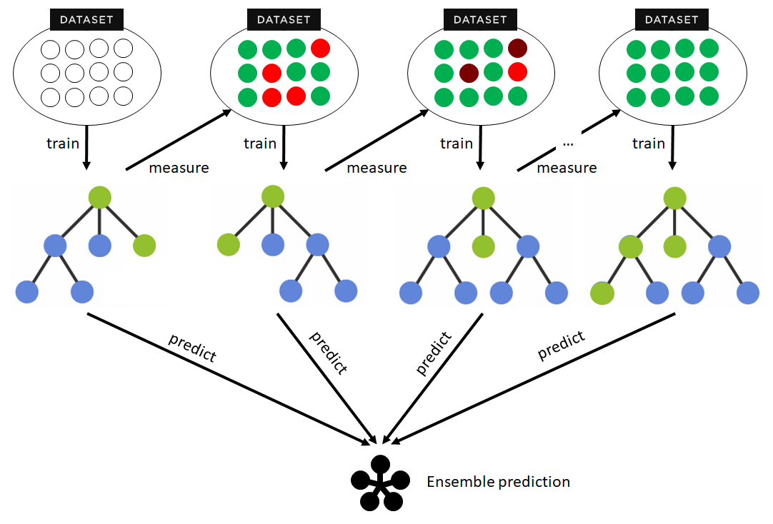
Boosting is a technique used to improve the performance of models. The essential idea behind boosting is to train a series of weak models (usually decision trees), each of which attempts to correct the errors of the previous one.

Structure

The model has a sequential structure and each model in the sequence is built to correct the errors of its predecessor. The structure of a boosting algorithm follows a process characterized by the following steps:

1. Initialization. First, an initial weight is assigned to each instance (row) in the training set. Generally, these weights are equal for all instances at startup.
2. Training the first model. A model is trained with the training data. This model will make some correct and some incorrect predictions.
3. Error calculation. Next, the error of the previous model is calculated based on the previous weights. Instances misclassified by this model will receive a higher weight, so they will be highlighted in the next step.
4. Training the second model. A new model is trained, but now it focuses more on the instances with higher weights (the ones that the previous model misclassified).
5. Iteration. Steps 3 and 4 are repeated for a predefined number of times, or until an acceptable error limit is reached. Each new model concentrates on correcting the errors of the previous model.
6. Combination of the models. After the end of the iterations, the models are combined through a weighted sum of their predictions. Models that perform better (i.e., make fewer errors in their predictions) are usually weighted more heavily in the sum.

It is important to keep in mind that boosting can be more susceptible to overfitting than other techniques if left unchecked, since each new model is trying to correct the errors of the previous one and could end up overfitting the training data. Therefore, it is crucial to have good control of the hyperparameters and to perform cross-validation during training.

Implementations

There are a multitude of implementations of this model, from more to less efficient, with more or less flexibility with respect to data types, depending on whether they are used for classification or regression, and so on. We will focus on gradient boosting, which is valid for both classification and regression.

XGBoost

XGBoost (eXtreme Gradient Boosting) is the most efficient implementation of the gradient boosting algorithm. It has been developed for speed and accuracy, and so far it is the best implementation, outperforming sklearn in training times. The time reduction is due to the fact that it provides methods to parallelize the tasks, flexibility when training the model and it is more robust, being able to include tree pruning mechanisms to save processing time. Whenever available, this is the alternative to sklearn that should be used.

In the reading we exemplified how to use XGBoost, but here we will provide a simple sample code to show you how to use sklearn to implement boosting:

Classification

1from sklearn.ensemble import GradientBoostingClassifier
2
3# Load of train and test data
4# These data must have been standardized and correctly processed in a complete EDA
5
6model = GradientBoostingClassifier(n_estimators = 5, random_state = 42)
7
8model.fit(X_train, y_train)
9
10y_pred = model.predict(y_test)

Regression

1from sklearn.ensemble import GradientBoostingRegressor
2
3# Load of train and test data
4# These data must have been standardized and correctly processed in a complete EDA
5
6model = GradientBoostingRegressor(n_estimators = 5, random_state = 42)
7
8model.fit(X_train, y_train)
9
10y_pred = model.predict(y_test)

Model hyperparameterization

We can easily build a decision tree in Python using the scikit-learn library and the GradientBoostingClassifier and GradientBoostingRegressor functions. We can also make use of a more efficient alternative called XGBoost to classify and regress with the XGBClassifier and XGBRegressor functions. Some of its most important hyperparameters and the first ones we should focus on are:

• n_estimators (n_estimators in XGBoost): This is probably the most important hyperparameter. It defines the number of decision trees in the forest. In general, a larger number of trees increases the accuracy and makes the predictions more stable, but it can also slow down the computation time considerably.
• learning_rate (learning_rate in XGBoost): The rate at which the model is accepted at each boosting stage. A higher learning rate may lead to a more complex model, while a lower rate will require more trees to obtain the same level of complexity.
• loss (objective in XGBoost): The loss function to optimize (amount of classification errors or difference with reality in regression).
• subsample (subsample in XGBoost): The fraction of instances to use to train the models. If it is less than 1.0, then each tree is trained with a random fraction of the total number of instances in the training dataset.
• max_depth (max_depth in XGBoost): The maximum depth of the trees. This is essentially how many splits the tree can make before making a prediction.
• min_samples_split (gamma in XGBoost): The minimum number of samples needed to split a node in each tree. If set to a high value, it prevents the model from learning too specific relationships and thus helps prevent overfitting.
• min_samples_leaf (min_child_weight in XGBoost): The minimum number of samples to have in a leaf node in each tree.
• max_features (colsample_by_level in XGBoost): The maximum number of features to consider when looking for the best split within each tree. For example, if we have 10 features, we can choose to have each tree consider only a subset of them when deciding where to split.

As we can see, only the first four hyperparameters refer to boosting, while the rest were truncated to decision trees. Another very important hyperparameter is the random_state, which controls the random generation seed. This attribute is crucial to ensure replicability.

Boosting vs. random forest

Boosting and random forest are two Machine Learning techniques that combine multiple models to improve the accuracy and stability of predictions. Although both techniques are based on the idea of assembling several models, they have some key differences.

	Boosting	Random forest
Ensemble strategy	Models are trained sequentially, each attempting to correct the errors of the previous model.	Models are trained independently, each with a random sample of the data.
Modeling capability	Can capture complex, nonlinear relationships in the data.	More "flat" and less ability to capture complex, nonlinear relationships.
Overfit prevention	May be more prone to overfitting, especially with noise or outliers in the data.	Generally less prone to overfitting.
Performance and accuracy	Tends to have higher accuracy performance, but may be more sensitive to hyperparameters.	May have lower precision performance, but is more robust to hyperparameter variations.
Training time	May be slower to train because models must be trained sequentially, one after another.	May be faster to train because all models can be trained in parallel.

These fundamental differences between the two models make them more or less suitable depending on the situation and the characteristics of the data. However, to make it clearer, we can establish some criteria based on the characteristics of the data that we could consider when choosing boosting and random forest:

	Boosting	Random forest
Data set size	Works best with large data sets where the improvement in performance can compensate for the additional training and tuning time.	Works well with both small and large sets, although it may be preferable for small data sets due to its efficiency.
Number of predictors	Performs best with large volumes of predictors, as it can capture complex interactions.	Works well with large volumes of predictors.
Distributions	Can handle unusual distributions as it is good at interpreting complex nonlinear relationships between data.	Robust to usual distributions, but may have problems modeling complex nonlinear relationships.
Outliers	Very sensitive to outliers.	Robust to outliers due to its partition-based nature.

The choice between boosting and random forest depends on the specific problem and data set you are working with, but these general rules are a good starting point for tackling different real-world problems.